HyPlan Tutorial: End-to-End Airborne Campaign Planning

This notebook walks through a complete airborne imaging spectroscopy campaign plan — from defining the sensor and aircraft, through generating flight lines over a study area, to producing an optimized flight plan with maps and altitude profiles. It is the recommended starting point for new HyPlan users.

Detail	Value
Audience	New HyPlan users, airborne campaign planners
Runtime	< 1 minute
Requires internet	No (uses bundled example data)
Credentials required	None
Optional dependencies	folium (interactive map)
Uses example data	Yes — Santa Catalina Island GeoJSON

What You Will Learn

• How to configure an instrument and aircraft for flight planning

• How to generate parallel flight lines that cover a study-area polygon

• How to check solar illumination constraints for imaging spectroscopy

• How to find nearby airports and optimize the flight line sequence

• How to compute a segment-by-segment flight plan with timing and distances

• How to visualize the plan on static plots and an interactive map

High-Level Workflow

Instrument ──► Aircraft ──► Study Area ──► Flight Lines ──► Solar Check
                                                                │
          Export ◄── Visualize ◄── Flight Plan ◄── Optimize ◄──┘
                                                   (airports)

Each section below corresponds to one step in this pipeline.

What This Notebook Produces

By the end of this notebook you will have:

1. Flight lines — a set of parallel survey lines covering Santa Catalina Island with 20% swath overlap

2. A flight plan table — segment-by-segment breakdown with distances, times, and altitudes

3. A static map — showing the complete route from takeoff through data collection to landing

4. An altitude profile — showing climb, cruise, and descent phases

5. An interactive map — a Folium map with clickable flight lines and metadata

# Core imports — HyPlan modules and standard scientific Python
import warnings
warnings.filterwarnings("ignore", category=FutureWarning)

import hyplan
from hyplan import (
    FlightLine, box_around_polygon,
    KingAirB200, AVIRIS3,
    Airport, initialize_data, airports_within_radius,
    compute_flight_plan, plot_flight_plan, plot_altitude_trajectory,
    build_graph, greedy_optimize,
    generate_swath_polygon, calculate_swath_widths,
    map_flight_lines, ureg,
)
from hyplan.sun import solar_threshold_times, solar_position_increments
from hyplan.geometry import haversine

import geopandas as gpd
import matplotlib.pyplot as plt

import matplotlib
from IPython.display import display


def _show_plot():
    """Display matplotlib figures without Agg-backend warnings."""
    if matplotlib.get_backend().lower() == "agg":
        for num in plt.get_fignums():
            display(plt.figure(num))
    else:
        getattr(plt, "show")()
import numpy as np
from shapely.geometry import shape
import json

1. Define the Instrument and Aircraft

Every flight plan starts with two objects: an instrument (the sensor being flown) and an aircraft (the platform carrying it). Together they determine the spatial resolution, swath width, ground speed, and altitude constraints that shape every downstream decision.

We will use AVIRIS-3, NASA’s next-generation imaging spectrometer, flown on a Beechcraft King Air B200.

sensor = AVIRIS3()
aircraft = KingAirB200()

print(f"Sensor:   {sensor.name}")
print(f"  FOV:    {sensor.fov}°")
print(f"  Pixels: {sensor.across_track_pixels} across-track")
print(f"  Rate:   {sensor.frame_rate}")
print()
print(f"Aircraft: {aircraft.aircraft_type}")
print(f"  Cruise: {aircraft.cruise_speed_at(aircraft.service_ceiling * 0.75).to(ureg.knot)}")
print(f"  Ceiling: {aircraft.service_ceiling}")

Sensor:   AVIRIS 3
  FOV:    39.6°
  Pixels: 1234 across-track
  Rate:   216.0 hertz

Aircraft: King Air 200
  Cruise: 238.5 knot
  Ceiling: 30000 foot

Sensor Performance at Altitude

The instrument’s spatial resolution (ground sample distance, GSD) and swath width both scale with the flight altitude above ground level (AGL). Flying higher gives a wider swath (fewer flight lines needed) but coarser pixels. This trade-off is central to campaign design.

altitudes_ft = [5000, 10000, 15000, 20000, 25000]
print(f"{'Altitude (ft)':>14s}  {'GSD (m)':>8s}  {'Swath (km)':>10s}")
print("-" * 36)
for alt_ft in altitudes_ft:
    alt = ureg.Quantity(alt_ft, "feet")
    gsd = sensor.ground_sample_distance(alt).to(ureg.meter)
    swath = sensor.swath_width(alt).to(ureg.kilometer)
    print(f"{alt_ft:>14d}  {gsd.magnitude:>8.2f}  {swath.magnitude:>10.2f}")

 Altitude (ft)   GSD (m)  Swath (km)
------------------------------------
          5000      0.85        1.10
         10000      1.71        2.19
         15000      2.56        3.29
         20000      3.41        4.39
         25000      4.27        5.49

Interpretation: At 20,000 ft AGL the GSD is about 3.4 m and the swath is roughly 4.4 km wide. For Santa Catalina Island (approximately 13 km across at its widest), this means we need only a handful of flight lines to achieve full coverage. Lower altitudes would improve resolution but require many more lines and more flight time.

2. Define the Study Area

The study area is specified as a polygon — typically loaded from a GeoJSON or shapefile. HyPlan uses this polygon to determine the optimal flight line heading and to calculate how many lines are needed for full coverage.

We load a GeoJSON for Santa Catalina Island, one of the Channel Islands off Southern California.

with open("../notebooks/exampledata/catalina.geojson") as f:
    geojson = json.load(f)

study_area = shape(geojson["features"][0]["geometry"])
centroid = study_area.centroid

print(f"Study area centroid: {centroid.y:.4f}°N, {centroid.x:.4f}°W")
print(f"Bounding box: {study_area.bounds}")

# Quick plot
fig, ax = plt.subplots(figsize=(8, 5))
gpd.GeoSeries([study_area]).plot(ax=ax, alpha=0.3, edgecolor="black")
ax.set_title("Santa Catalina Island")
ax.set_xlabel("Longitude")
ax.set_ylabel("Latitude")
plt.tight_layout()
_show_plot()

Study area centroid: 33.3821°N, -118.4332°W
Bounding box: (-118.6064373, 33.2987495, -118.3035159, 33.479031)

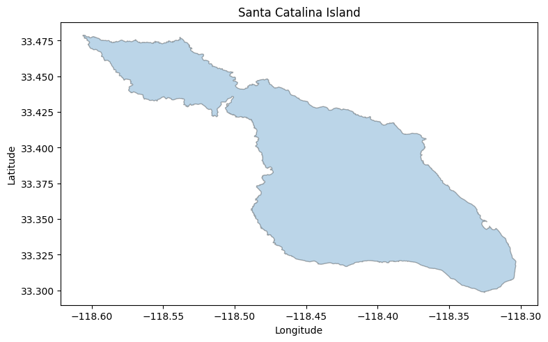
Interpretation: The island is elongated roughly WNW-ESE. HyPlan’s box_around_polygon will detect this orientation automatically and align flight lines along the long axis, minimizing the number of lines required for full coverage.

3. Generate Flight Lines

A flight line is a straight-line segment the aircraft flies while the instrument collects data. box_around_polygon generates a set of parallel flight lines that cover the study area, with a specified percentage of swath overlap between adjacent lines.

Key parameters:

• altitude_msl — flight altitude in mean sea level (MSL); determines GSD and swath width

• overlap — percentage of swath overlap between adjacent lines (20% is typical for imaging spectroscopy)

• alternate_direction — if True, adjacent lines are flown in opposite directions to reduce transit time

flight_altitude = ureg.Quantity(20000, "feet")

flight_lines = box_around_polygon(
    instrument=sensor,
    altitude_msl=flight_altitude,
    polygon=study_area,
    box_name="SRI",
    overlap=20.0,
    alternate_direction=True,
    clip_to_polygon=False,
)

print(f"Generated {len(flight_lines)} flight lines at {flight_altitude}")
for fl in flight_lines:
    print(f"  {fl.site_name}: length={fl.length.to(ureg.kilometer):.1f}, azimuth={fl.az12.magnitude:.1f}°")

Generated 4 flight lines at 20000 foot
  SRI_L01_FL200: length=33.4 kilometer, azimuth=295.6°
  SRI_L02_FL200: length=33.4 kilometer, azimuth=115.4°
  SRI_L03_FL200: length=33.4 kilometer, azimuth=295.6°
  SRI_L04_FL200: length=33.5 kilometer, azimuth=115.4°

# Plot flight lines with swath polygons over the study area
fig, ax = plt.subplots(figsize=(10, 6))
gpd.GeoSeries([study_area]).plot(ax=ax, alpha=0.2, edgecolor="black", color="lightgreen")

for fl in flight_lines:
    # Draw swath polygon
    swath = generate_swath_polygon(fl, sensor)
    gpd.GeoSeries([swath]).plot(ax=ax, alpha=0.15, color="blue", edgecolor="steelblue", linewidth=0.5)
    # Draw flight line
    x, y = fl.geometry.xy
    ax.plot(x, y, "b-", linewidth=1.5, alpha=0.7)
    ax.annotate(fl.site_name, xy=(x[0], y[0]), fontsize=7, color="navy")

ax.set_title(f"Flight Lines and Swath Coverage over Santa Catalina Island ({len(flight_lines)} lines)")
ax.set_xlabel("Longitude")
ax.set_ylabel("Latitude")
plt.tight_layout()
_show_plot()

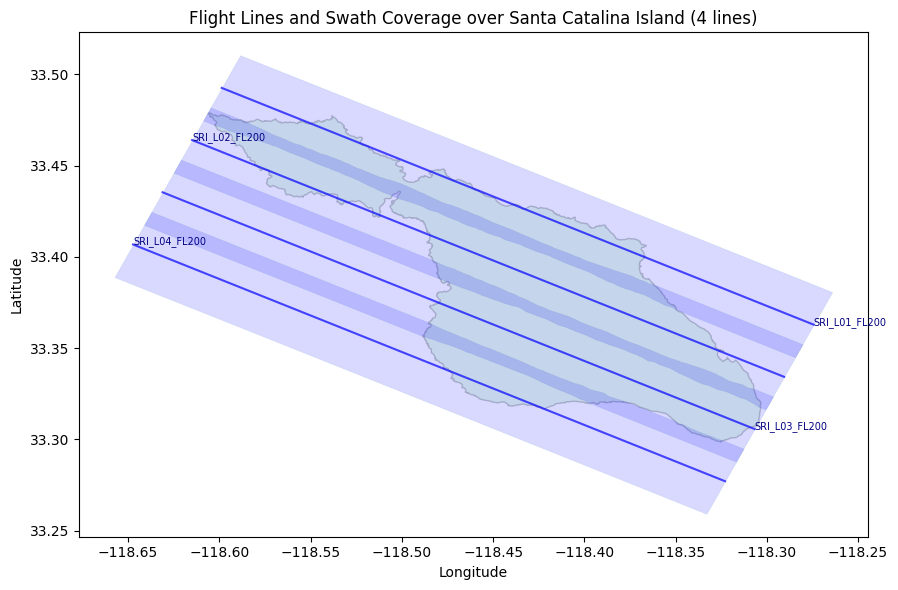
Interpretation: The four flight lines are aligned along the long axis of the island (approximately 296 / 115 degrees). The blue shaded swath footprints overlap slightly, ensuring no gaps in spatial coverage. Adjacent lines alternate direction (note the alternating azimuths of ~296 and ~115 degrees), which reduces transit time between lines.

Swath Geometry

Each flight line has a ground swath footprint — the area on the ground actually imaged by the sensor. The swath width varies slightly along the line due to Earth curvature. We can verify that the computed footprint matches the theoretical swath width.

# Compute swath for the first flight line
swath_poly = generate_swath_polygon(flight_lines[0], sensor)
widths = calculate_swath_widths(swath_poly)

print(f"Swath widths for {flight_lines[0].site_name}:")
print(f"  Min:  {widths['min_width']:.0f} m")
print(f"  Mean: {widths['mean_width']:.0f} m")
print(f"  Max:  {widths['max_width']:.0f} m")

# Compare with theoretical swath width
theoretical = sensor.swath_width(flight_altitude).to(ureg.meter).magnitude
print(f"\nTheoretical swath width at {flight_altitude}: {theoretical:.0f} m")

Swath widths for SRI_L01_FL200:
  Min:  4206 m
  Mean: 4314 m
  Max:  4389 m

Theoretical swath width at 20000 foot: 4389 m

Interpretation: The computed swath footprint (mean ~4,314 m) closely matches the theoretical value (4,389 m). The small difference arises because the footprint polygon accounts for Earth curvature along the flight line. This confirms the geometry calculations are consistent.

4. Check Solar Illumination

Imaging spectrometers require adequate solar illumination — shadows and low sun angles degrade data quality. The usable data-collection window is bounded by a minimum solar elevation angle (typically 30 degrees for acceptable data, 50 degrees for ideal conditions).

HyPlan computes the times when the sun crosses these elevation thresholds at the study area location.

# Solar elevation thresholds: 30° (minimum usable) and 50° (ideal)
solar_times = solar_threshold_times(
    latitude=centroid.y,
    longitude=centroid.x,
    start_date="2025-06-15",
    end_date="2025-06-20",
    thresholds=[30, 50],
    timezone_offset=-7,  # PDT
)

print("Solar threshold times (PDT):")
print(solar_times.to_string(index=False))

Solar threshold times (PDT):
      Date  Rise_30  Rise_50   Set_50   Set_30
2025-06-15 08:21:00 09:57:00 15:51:00 17:28:00
2025-06-16 08:21:00 09:58:00 15:52:00 17:28:00
2025-06-17 08:21:00 09:58:00 15:52:00 17:28:00
2025-06-18 08:22:00 09:58:00 15:52:00 17:28:00
2025-06-19 08:22:00 09:58:00 15:52:00 17:29:00
2025-06-20 08:22:00 09:58:00 15:53:00 16:59:00

Interpretation: In mid-June, the ideal collection window (solar elevation above 50 degrees) runs from roughly 10:00 to 15:50 local time — about 6 hours. The acceptable window (above 30 degrees) extends from 08:20 to 17:30, giving roughly 9 hours. For our 4-line plan requiring only ~1.3 hours of total flight time, solar constraints are not a limiting factor on any of these days.

# Detailed solar positions on June 15
positions = solar_position_increments(
    latitude=centroid.y,
    longitude=centroid.x,
    date="2025-06-15",
    min_elevation=20,
    timezone_offset=-7,
    increment="30min",
)

print("Solar positions on June 15, 2025 (elevation > 20°):")
print(positions.to_string(index=False))

Solar positions on June 15, 2025 (elevation > 20°):
    Time    Azimuth  Elevation
17:00:00 276.292407  35.741662
17:30:00 279.859509  29.543416
18:00:00 283.362259  23.411088
08:00:00  77.955958  25.764260
08:30:00  81.468844  31.924735
09:00:00  85.083684  38.142670
09:30:00  88.925483  44.395012
10:00:00  93.180355  50.654838
10:30:00  98.153939  56.885370
11:00:00 104.401870  63.026699
11:30:00 113.049055  68.961515
12:00:00 126.606069  74.412980
12:30:00 150.412844  78.625442
13:00:00 187.395858  79.883538
13:30:00 220.208569  77.274189
14:00:00 239.343734  72.451360
14:30:00 250.611315  66.766772
15:00:00 258.163652  60.734407
15:30:00 263.841954  54.550464
16:00:00 268.498077  48.304093
16:30:00 272.570389  42.044117

Interpretation: Peak solar elevation (~80 degrees) occurs around 13:00 local time. The solar azimuth sweeps from east (~78 degrees) in the morning to west (~283 degrees) in the evening. For sun-glint-sensitive applications (e.g., aquatic targets), you would avoid flight headings that align with the solar azimuth. See the solar_planning and glint_analysis notebooks for more detail.

5. Find Nearby Airports

The flight plan needs a departure and return airport, and possibly refueling stops for longer campaigns. HyPlan includes a built-in airport database that can be searched by proximity to the study area.

# Initialize airport database for the US
initialize_data(countries=["US"])

# Find airports within 150 km of the study area
nearby = airports_within_radius(
    centroid.y, centroid.x,
    radius=150,
    unit="kilometers",
    return_details=True,
)

nearby["distance_km"] = nearby["distance_m"] / 1000.0

print(f"Found {len(nearby)} airports within 150 km:")
print(nearby[["icao_code", "name", "municipality", "distance_km"]].head(10).to_string(index=False))

Found 53 airports within 150 km:
icao_code                                              name        municipality  distance_km
     KAVX                                  Catalina Airport              Avalon     3.001566
     KNUC San Clemente Island Naval Auxiliary Landing Field San Clemente Island    42.474291
     KTOA                                   Zamperini Field            Torrance    47.639764
     KLGB                  Long Beach International Airport          Long Beach    54.977377
     KSLI                       Los Alamitos Army Air Field        Los Alamitos    57.656498
     KCPM                           Compton Woodley Airport             Compton    59.134582
     KHHR   Jack Northrop Field Hawthorne Municipal Airport           Hawthorne    60.810731
     KSNA    John Wayne Orange County International Airport           Santa Ana    61.596349
     KLAX                 Los Angeles International Airport         Los Angeles    62.361719
     KFUL                       Fullerton Municipal Airport           Fullerton    68.766749

Interpretation: The closest airport is Catalina (KAVX) on the island itself, but it has a short runway unsuitable for the King Air B200 with full fuel and instruments. In practice, we select airports based on runway length, fuel availability, and hangar space for the aircraft and instrument team. Here we choose Santa Barbara (KSBA) as the base airport, with Oxnard (KOXR) as a backup refueling option.

# Select departure and return airports
departure_airport = Airport("KSBA")  # Santa Barbara
return_airport = Airport("KSBA")

# Additional refueling option
refuel_airport = Airport("KOXR")  # Oxnard (Ventura County)

airports = [departure_airport, refuel_airport]

print(f"Departure: {departure_airport.name} ({departure_airport.icao_code})")
print(f"  Location: {departure_airport.latitude:.4f}°N, {departure_airport.longitude:.4f}°W")
print(f"  Elevation: {departure_airport.elevation_ft:.0f} ft")
print(f"\nRefuel option: {refuel_airport.name} ({refuel_airport.icao_code})")

Departure: Santa Barbara Municipal Airport (KSBA)
  Location: 34.4262°N, -119.8400°W
  Elevation: 13 ft

Refuel option: Oxnard Airport (KOXR)

6. Optimize Flight Line Sequence

Given a set of flight lines and airport locations, the optimizer finds an efficient ordering that minimizes total transit time. It respects operational constraints such as maximum aircraft endurance per sortie and maximum daily flight time, inserting refueling stops or multi-day breaks as needed.

result = greedy_optimize(
    aircraft=aircraft,
    flight_lines=flight_lines,
    airports=airports,
    takeoff_airport=departure_airport,
    return_airport=return_airport,
    max_endurance=4.5,           # hours per sortie
    max_daily_flight_time=8.0,   # hours per day
    max_days=3,
)

print(f"Optimization result:")
print(f"  Lines covered: {result['lines_covered']}/{len(flight_lines)}")
print(f"  Total time:    {result['total_time']:.2f} hours")
print(f"  Days used:     {result['days_used']}")
for i, dt in enumerate(result["daily_times"], 1):
    print(f"    Day {i}: {dt:.2f} hours")
print(f"  Refuel stops:  {result['refuel_stops']}")
print(f"\nRoute: {' → '.join(result['route'])}")

Optimization result:
  Lines covered: 4/4
  Total time:    1.22 hours
  Days used:     1
    Day 1: 1.22 hours
  Refuel stops:  []

Route: KSBA → SRI_L02_FL200_start → SRI_L02_FL200_end → SRI_L03_FL200_start → SRI_L03_FL200_end → SRI_L04_FL200_start → SRI_L04_FL200_end → SRI_L01_FL200_start → SRI_L01_FL200_end → KSBA

Interpretation: All four flight lines fit in a single sortie of about 1.3 hours — well within the 4.5-hour endurance limit. No refueling stops are needed. The optimizer chose to fly L02 first (nearest to the inbound route from KSBA), then proceed through L03, L04, and L01 before returning. For larger campaigns with dozens of lines, the optimizer becomes essential for minimizing wasted transit time across multiple days.

7. Compute the Flight Plan

The flight plan converts the optimized sequence into a detailed, segment-by-segment table. Each segment has a type (takeoff, transit, flight_line, descent), distance, and estimated time. This is the primary deliverable for the flight crew and campaign management team.

flight_plan = compute_flight_plan(
    aircraft=aircraft,
    flight_sequence=result["flight_sequence"],
    takeoff_airport=departure_airport,
    return_airport=return_airport,
)

print(f"Flight plan: {len(flight_plan)} segments")
print()
cols = ["segment_type", "segment_name", "distance", "time_to_segment"]
print(flight_plan[cols].to_string(index=False))

Flight plan: 11 segments

segment_type                   segment_name  distance  time_to_segment
     takeoff                      Departure 50.182689        15.470181
     transit                      Departure 29.140306         7.315558
 flight_line                  SRI_L02_FL200 24.051540         6.038044
     transit SRI_L02_FL200 to SRI_L03_FL200  9.961892         2.500893
 flight_line                  SRI_L03_FL200 24.057438         6.039524
     transit SRI_L03_FL200 to SRI_L04_FL200 10.058368         2.525113
 flight_line                  SRI_L04_FL200 24.063402         6.041021
     transit SRI_L04_FL200 to SRI_L01_FL200 10.155258         2.549437
 flight_line                  SRI_L01_FL200 24.045693         6.036576
     transit                         Return 37.610919         9.442072
     descent                         Return 52.148004        13.993382

# Summary statistics
total_distance = flight_plan["distance"].sum()
total_time = flight_plan["time_to_segment"].sum()
data_segments = flight_plan[flight_plan["segment_type"] == "flight_line"]
data_distance = data_segments["distance"].sum()
data_time = data_segments["time_to_segment"].sum()

print(f"Total distance:      {total_distance:.1f} nmi")
print(f"Total flight time:   {total_time:.1f} min")
print(f"Data collection:     {data_distance:.1f} nmi ({data_time:.1f} min)")
print(f"Collection fraction: {data_time/total_time*100:.1f}%")

Total distance:      295.5 nmi
Total flight time:   78.0 min
Data collection:     96.2 nmi (24.2 min)
Collection fraction: 31.0%

Interpretation: The collection fraction (about 32%) tells us that roughly one-third of the total flight time is spent actually collecting data. The remainder is transit to/from the airport and turns between flight lines. This is typical for island targets that require significant ferry time. For study areas closer to the departure airport, the collection fraction would be higher.

8. Visualize

HyPlan provides several visualization functions. The flight plan map shows the complete route; the altitude profile shows the vertical trajectory; and the interactive map allows exploration of individual flight lines.

Flight Plan Map

plot_flight_plan(
    flight_plan,
    departure_airport,
    return_airport,
    result["flight_sequence"],
)

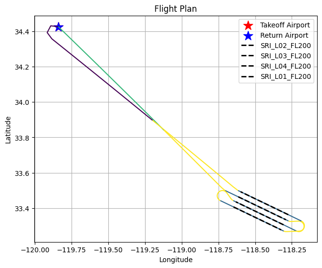
Interpretation: The map shows the complete route: departure from KSBA, transit to the study area, four data-collection legs over the island, and return to KSBA. The parallel flight lines are clearly visible over the island, with short transit segments connecting them.

Altitude Profile

plot_altitude_trajectory(flight_plan, aircraft=aircraft)

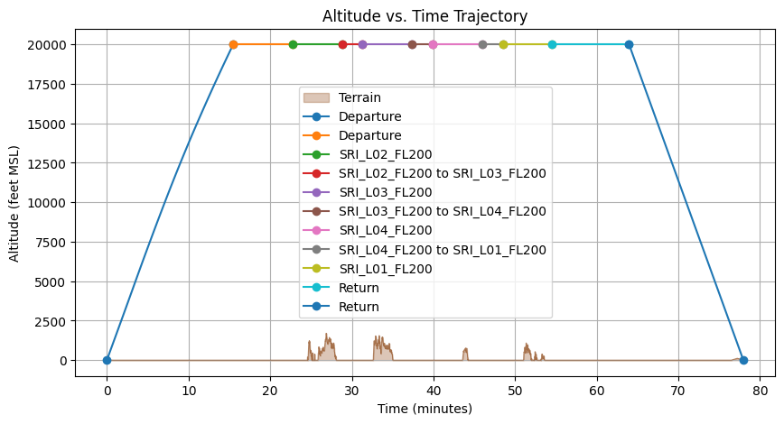
Interpretation: The altitude profile shows the aircraft climbing from the airport to the survey altitude of 20,000 ft MSL, maintaining altitude during data collection, and descending back to the airport. The flat segments at cruise altitude correspond to the four flight lines and their connecting transits.

Interactive Map

The Folium-based interactive map lets you zoom, pan, and click on individual flight lines to inspect their metadata (name, altitude, heading, length). This is useful for sharing plans with collaborators or reviewing coverage in detail.

m = map_flight_lines(
    result["flight_sequence"],
    center=(centroid.y, centroid.x),
    zoom_start=10,
)
m

Make this Notebook Trusted to load map: File -> Trust Notebook

9. Create Individual Flight Lines

For cases where you need to define flight lines manually — for example, specific transects, calibration lines, or lines that do not follow a regular grid — HyPlan provides two factory methods:

• start_length_azimuth — define a line from its start point, length, and heading (ground track azimuth)

• center_length_azimuth — define a line from its center point, extending equally in both directions

You can also split long lines into shorter segments with gaps between them (useful for instrument calibration or data-volume constraints).

# From a start point, length, and heading
transect = FlightLine.start_length_azimuth(
    lat1=34.0, lon1=-119.8,
    length=ureg.Quantity(30, "kilometer"),
    az=270.0,
    altitude_msl=ureg.Quantity(20000, "feet"),
    site_name="Coastal Transect",
)

print(f"{transect.site_name}:")
print(f"  Start: ({transect.lat1:.4f}, {transect.lon1:.4f})")
print(f"  End:   ({transect.lat2:.4f}, {transect.lon2:.4f})")
print(f"  Length: {transect.length.to(ureg.kilometer):.2f}")
print(f"  Heading: {transect.az12.magnitude:.1f}°")

Coastal Transect:
  Start: (34.0000, -119.8000)
  End:   (33.9996, -120.1247)
  Length: 30.00 kilometer
  Heading: 270.0°

# From a center point (extends equally in both directions)
centered = FlightLine.center_length_azimuth(
    lat=34.0, lon=-119.8,
    length=ureg.Quantity(30, "kilometer"),
    az=0.0,
    altitude_msl=ureg.Quantity(20000, "feet"),
    site_name="N-S Transect",
)

print(f"{centered.site_name}:")
print(f"  Start: ({centered.lat1:.4f}, {centered.lon1:.4f})")
print(f"  End:   ({centered.lat2:.4f}, {centered.lon2:.4f})")
print(f"  Center: ({(centered.lat1+centered.lat2)/2:.4f}, {(centered.lon1+centered.lon2)/2:.4f})")

N-S Transect:
  Start: (33.8648, -119.8000)
  End:   (34.1352, -119.8000)
  Center: (34.0000, -119.8000)

# Split a long line into segments
segments = transect.split_by_length(
    max_length=ureg.Quantity(10, "kilometer"),
    gap_length=ureg.Quantity(1, "kilometer"),
)
print(f"Split into {len(segments)} segments:")
for seg in segments:
    print(f"  {seg.site_name}: {seg.length.to(ureg.kilometer):.2f}")

Split into 3 segments:
  Coastal Transect_seg_0: 10.00 kilometer
  Coastal Transect_seg_1: 10.00 kilometer
  Coastal Transect_seg_2: 8.00 kilometer

10. Unit Conversions

Aviation and remote sensing mix unit systems freely — altitudes in feet, distances in nautical miles or kilometers, speeds in knots, and angles in degrees or radians. HyPlan uses pint for unit-safe arithmetic throughout, and provides convenience helpers for quick conversions.

from hyplan.units import convert_angle, convert_time

print(f"180° in radians: {convert_angle(180.0, 'degrees', 'radians'):.4f}")
print(f"1 rad in degrees: {convert_angle(1.0, 'radians', 'degrees'):.4f}")
print(f"90 min in hours: {convert_time(90.0, 'minutes', 'hours')}")
print(f"2 days in seconds: {convert_time(2.0, 'days', 'seconds'):.0f}")

180° in radians: 3.1416
1 rad in degrees: 57.2958
90 min in hours: 1.5
2 days in seconds: 172800

Summary

This tutorial demonstrated the core HyPlan workflow:

Step	Function	Purpose
Instrument setup	AVIRIS3()	Define sensor characteristics
Aircraft setup	KingAirB200()	Define aircraft performance
Flight box	box_around_polygon()	Generate parallel flight lines
Solar check	solar_threshold_times()	Determine illumination windows
Airport search	airports_within_radius()	Find nearby airports
Optimization	greedy_optimize()	Order lines for efficiency
Flight plan	compute_flight_plan()	Detailed segment-by-segment plan
Visualization	plot_flight_plan(), map_flight_lines()	Maps and altitude profiles

Final Outputs

Output	Description
4 flight lines	Parallel survey lines covering Santa Catalina Island at 20,000 ft MSL
Flight plan table	9 segments with distances (nmi) and times (min)
Static map	Complete route from KSBA to study area and back
Altitude profile	Vertical trajectory showing climb, cruise, and descent
Interactive map	Folium map with clickable flight line metadata

---

Operational Takeaways

• Solar windows matter. For mid-latitude summer campaigns, the usable imaging window is roughly 6 hours (50+ degree solar elevation). Winter campaigns or high-latitude sites will have much shorter windows.

• Collection fraction is typically 20-40%. Most flight time is spent on transit and turns, not data collection. Choosing an airport closer to the study area improves efficiency.

• Swath overlap is a trade-off. More overlap means better mosaicking quality but more flight lines (and cost). 20% is a common starting point for imaging spectroscopy.

• Altitude drives resolution and coverage. Higher altitude gives wider swath (fewer lines) but coarser pixels. Match the altitude to your science requirements.

• The optimizer saves real money. For large campaigns with 50+ lines across multiple days, automated sequencing can reduce total flight hours by 10-20% compared to manual ordering.

Common Pitfalls

• MSL vs AGL confusion. HyPlan flight altitudes are specified in MSL (mean sea level). Over elevated terrain, the altitude AGL (above ground level) — and therefore the GSD — will be different from what you compute using MSL alone. See the terrain_aware_planning notebook.

• Heading vs ground track. A flight line’s azimuth is its ground track direction, not the aircraft heading. In the presence of crosswinds, the aircraft heading will differ from the ground track to maintain the desired line. See the winds and wind_effects notebooks.

• Wind-from vs wind-to. Meteorological convention reports wind as the direction it blows from (e.g., “a westerly wind” blows from west to east). HyPlan follows this convention. Do not confuse it with the direction the wind is blowing toward.

• Feet vs meters. Aviation altitudes are in feet; scientific products typically use meters. Always check units when converting between flight planning and science contexts. HyPlan’s pint-based unit system helps prevent silent errors.

• Swath width vs footprint. “Swath width” is the cross-track ground distance for a single scan line at a given altitude. “Swath footprint” is the full 2D polygon traced out along the entire flight line. The footprint width varies slightly due to Earth curvature.

Next Steps

Explore these notebooks to dive deeper into specific aspects of campaign planning:

Notebook	Topic
flight_line_operations.ipynb	Creating, splitting, merging, and manipulating individual flight lines
flight_box_generation.ipynb	Advanced options for generating flight line grids over polygons
flight_plan_computation.ipynb	Detailed flight plan construction and segment analysis
flight_optimizer_demo.ipynb	Multi-day optimization with refueling and endurance constraints
winds.ipynb / wind_effects.ipynb	Incorporating wind into ground speed, heading, and timing calculations
solar_planning.ipynb	Detailed solar geometry and illumination window analysis
cloud_analysis.ipynb	Historical cloud-cover analysis for campaign scheduling
terrain_aware_planning.ipynb	Adjusting for terrain elevation (MSL to AGL corrections)
export_formats.ipynb	Exporting flight plans to KML, CSV, and pilot-ready formats
aircraft_performance.ipynb	Exploring aircraft climb rates, cruise speeds, and endurance

For more details, see the HyPlan documentation.